Printing large spreadsheets in Excel

Printing those monster Excel sheets

by The Guru

Taming the Large Spreadsheet: The Process

Once you’ve acquired some basic skills in Excel, the process for formatting a sheet to print is really pretty straightforward:

1. Setting the Print Area and Print Titles
2. Inserting Headers and Footers
3. Controlling Margins, Page Orientation, and Page Size
4. Inserting/Adjusting Page Breaks
5. Previewing the final result and tweaking where necessary

Let’s step through it.

Setting the Print Area and Print Titles

Right off the bat, you’re going to need to decide how much of the spreadsheet to print.

Most of the time, you need to print the entire thing.  But that doesn’t let you off the hook here.

That’s because, even if you want to print all the data (the Print Area), you’re probably going to want to print the row and column labels on each page (the Print Titles).

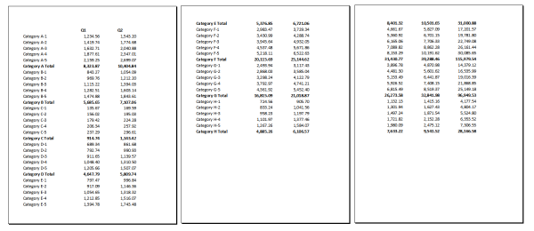
Let’s compare two printouts:

Printout 1

Pages 1, 2 and 4 of an Excel printout (click to enlarge)

If you look closely at these Print Preview images, page 1 is fine – you can see the column labels (with the fiscal quarter designations at the top) and the row labels (with the category names) on the left.  But then page 2 is missing the column labels, and if you look at page 4, none of that is carried over that far into the printout.  So, unless you’re planning on taping together your spreadsheet into one big piece of paper, you’re going to have a hard time figuring out which numbers go with each quarter/category.

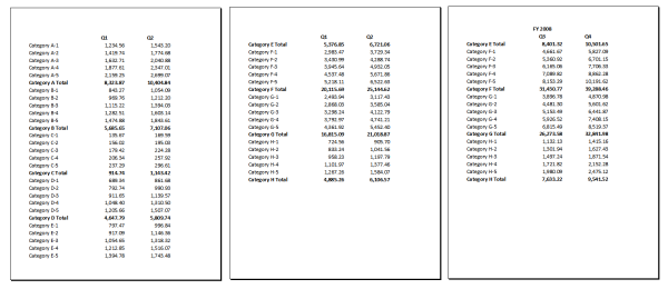
Compare that with Printout 2:

Pages 1, 2, & 4 from printout with changes

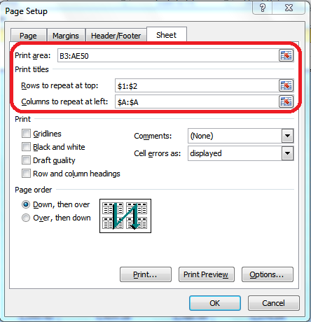
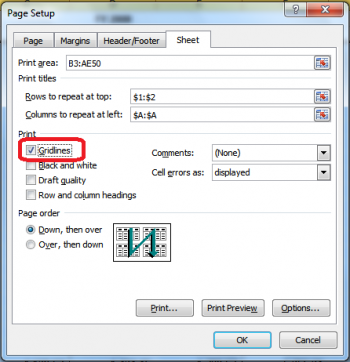
The difference here is that I’ve defined the print area as all of the numbers (from cell B3 to AE50) and the print titles as rows 1 and 2 and column A by going into the Page Setup dialog box from the Page Layout tab, then selecting the Sheet tab:

That’s what enables the row and column labels to print on every page.

Inserting Headers & Footers

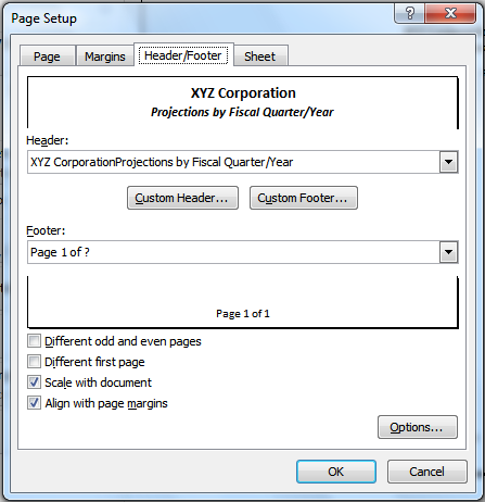
Once you’re in the Page Setup dialog box, you can define headers and footers to print on every page on the Header/Footer tab.  For example, you can insert a custom title at the top and page numbers at the bottom by clicking the Custom Header and Custom Footer buttons:

Controlling Margins, Page Orientation and Page Size

The printout is starting to look somewhat better, but there’s some further tweaking to be done here.  For instance, maybe the sheet makes more sense (and prints more attractively) printed landscape rather than portrait.  Or perhaps it’s a good idea to print this on Legal size paper (8.5″ x 14″) or even on Ledger size (11″ x 14″) rather than Letter (8.5″ x 11″).

Given we’re already in the Page Setup dialog box, we’ll just need to explore the other two tabs: Page and Margins.

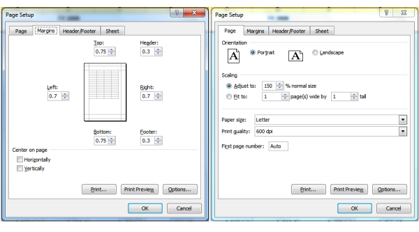As you can see from above, you can adjust the placement of the headers and footers and the page margins on the Margins tab, and control the orientation (portrait versus landscape) and the page size (letter, legal, ledger, A4, etc.) on the Page tab.  You can even scale the spreadsheet up or down by a set percentage, or force the spreadsheet to print on a particular configuration of pages across/down (if you want everything to fit on one page, you’d choose 1 page(s) wide by 1 page(s) tall, for example).

One more thing: if printing gridlines on your sheet would help improve readability (you know, borders around each cell to make following rows/columns easier), go back to the Sheet tab and check the Gridlines box:

Notice here, too, that you can also control whether the row and column headings (1, 2, 3 for rows, A, B, C for columns) print on your sheet.  Excel will also let you set whether the printout order goes horizontal then vertical or the other way around (in other words, whether you want the pages to print across, then down).

At any point, you can click Print Preview to check your progress.

Inserting/Adjusting Page Breaks

With some sheets, you may want to be sure that certain information appears together on a page.  In the sample sheet, it would probably make the information more readable to print all of a fiscal year’s information one sheet across.

You’re probably familiar with page breaks in Word.  Excel’s are different in one key respect: you can define page breaks horizontally and vertically.

The easiest way to deal with page breaks in Microsoft Excel is in Page Break Preview mode.  Go to the View tab on your ribbon and click Page Break Preview:

Excel will automatically place some page breaks for you.  In Page Break Preview mode, you can literally drag those pre-defined page breaks around on the screen until they’re placed where you want them.

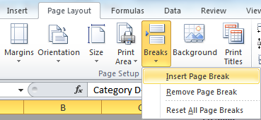
If you need to manually insert a page break within your Excel sheet, select the row or column directly after which you want to insert the break, then go to the Page Layout tab and, in the Page Setup section, click the drop-down under Breaks to insert the appropriate break:

If you make a mistake in where you insert your page break, simply drag the page break to the right spot (since you’re in Page Break Preview mode anyway).

Previewing and Adjusting the Final Print Result

At virtually any point in this process, you can go to Print Preview to check your progress and make a note of any adjustments you need to make.

If you’ve upgraded to version 2010 yet, you can also make adjustments directly in Print Preview:

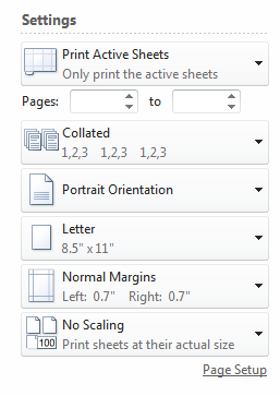The above menu appears directly to the left of the preview of your document.  You can make on-the-fly adjustments within this menu, or click Page Setup at the bottom to go back to the Page Setup dialog for more options.

The Final Result

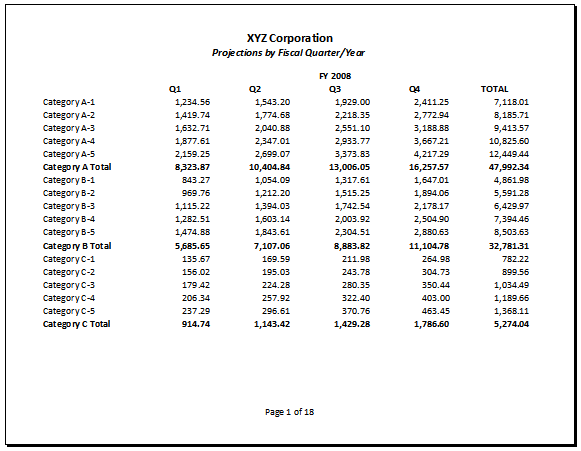
After all that, here’s how the sample spreadsheet finally prints:

The Video

Because these things sometimes are more easily explained by showing you step-by-step, I’ve added a video below, along with a downloadable transcript.

Here’s a link to the video: Excel-print-large-spreadsheets.mp4

And here’s the video transcript: Excel-Monster-Spreadsheet-Video-Transcript.pdf

Printing large spreadsheets in Microsoft Excel 2007-2010